Summarized example
Here we summarize the nine previous steps with the Python example executable we have used through the documentation.
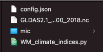
Our component takes as input a netcdf file and produces a netcdf file and a mp4 movie as a result. Parameters are passed through a configuration file. This is what the component folder looks like after we execute the first MIC command:
The sequence of commands required for encapsulating the model are:
- Start:
mic pkg start - Trace the execution command:
mic pkg trace python3 WM_climate_indices.py config.json -
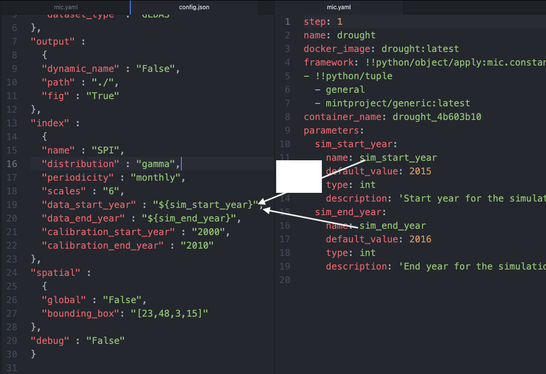
Expose the start/end years of the simulation with default values of 2015 and 2016 respectively:
-
mic pkg parameters -n sim_start_year -v 2015 -
mic pkg parameters -n sim_end_year -v 2016 -
Edit the configuration file to match the parameters name to their values in the
mic.yamlfile:
-
Select inputs to expose
-
Edit the configuration file to identify which input files should be added:
{
"data" :
  {
  "dataset_name" : "${input_nc}",
  "dataset_type" : "GLDAS"
},
"output" :
  {
  "dynamic_name" : "False",
  "path" : "./",
  "fig" : "True"
},
"index" :
  {
  "name" : "SPI",
  "distribution" : "gamma",
  "periodicity" : "monthly",
  "scales" : "6",
  "data_start_year" : "${sim_start_year}",
  "data_end_year" : "${sim_end_year}",
  "calibration_start_year" : "2000",
  "calibration_end_year" : "2010"
},
"spatial" :
  {
  "global" : "False",
  "bounding_box": "[23,48,3,15]"
},
"debug" : "False"
}
mic pkg inputs
- Select outputs to expose:
mic pkg outputs - Create wrapper:
mic pkg wrapper. - Run wrapper and verify results:
mic pkg run. Once you are done, exit the MIC environment: Typeexit - Upload:
mic pkg upload
Done!